Inverse Distance Weighting (IDW) Interpolation

---

“Inverse Distance Weighting (IDW) interpolation estimates unknown values with specifying search distance, closest points, power setting & barriers.”

---

How Inverse Distance Weighting (IDW) interpolation works

Whether you want to estimate the amount of rainfall or elevation in specific areas, you will probably want to learn about the different interpolation methods like inverse distance weighted.

To do this, you start with known values, and you estimate the unknown points through interpolation.

Inverse Distance Weighting (IDW) interpolation is mathematical (deterministic) assuming closer values are more related than further values with its function.

While good if your data is dense and evenly spaced, let’s look at how IDW works and where it works best.

First, a recap on interpolation

When you are given known values, interpolation estimates unknown values.

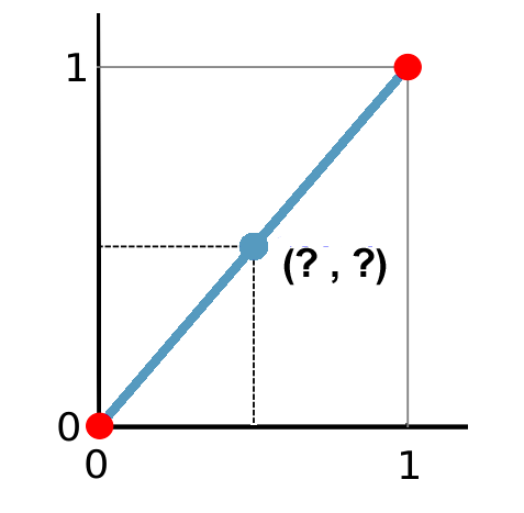
To estimate the point in between, draw a dotted line to the x-axis and then to the y-axis. A good estimate of the blue point is 0.5 and 0.5. You just did a linear interpolation.

Interpolation in GIS works the same. First, you take known points. Next, you create a surface by estimating unknown ones. Let’s examine this in a bit more detail.

Spatial interpolation and IDW

Near points are more alike than far points:

• Noise is louder closer to a siren than further away.
• When it’s raining, it’s more likely to rain 1 meter away compared to 500 meters away.

These are examples of spatial autocorrelation or Tobler’s First Law of Geography. Spatial autocorrelation is the underlying assumption of Inverse Distance Weighting.

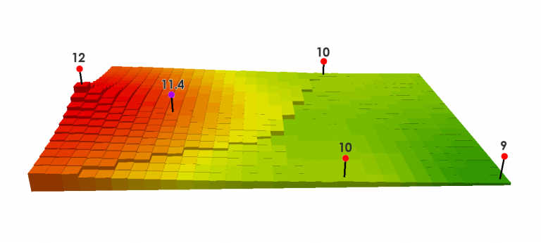
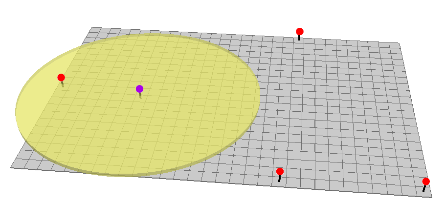
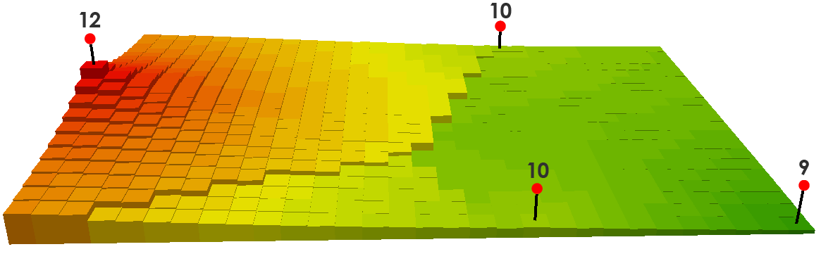
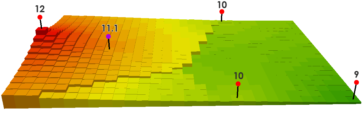
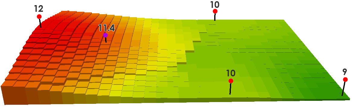
In the example below, the red points have known elevation values. The other points will be interpolated. If you wanted to measure the purple point, you can set up your interpolation so that it takes a fixed or variable number of points. In this example, it uses a fixed number of points of 3 and uses the three closest points.

You can see how IDW is a very flexible spatial interpolation method. You can set up your IDW interpolation in different ways. Specify your search radius and your interpolation will only use the number of known points within your search radius.

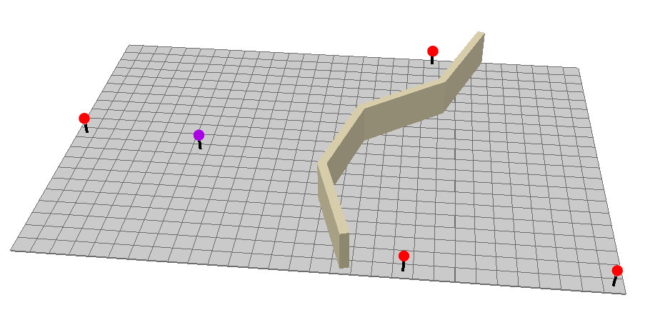
Another reason why IDW interpolation is so flexible is that you can set up barriers. If there are ridges in an elevation profile or noise barriers – then these are appropriate examples to use a barrier. This polyline barrier prevents it from searching for the input sample points.

Tweaking the results with power settings

Now, that you know how to set up search distances, select the number of points, and use barriers, it’s time to learn about the power settings in IDW. This is best illustrated with an example.

Interpolated points are estimated based on their distance from known cell values. Points that are closer to known values will be more influenced than points that are farther away.

If you have a power of 1, it smooths out the interpolated surface.

If you have a power of 2, it increases the overall influence it has on the known values. You can see how the peaks and values are more localized and are not averaged out as much as a power of 1.

The math behind Inverse Distance Weighting

There’s nothing to be afraid of with IDW math. Remember that the search distance or the number of closest points determines how many points will be used.

We use the 3 closest points in this example:

Here’s what the table looks like for these 3 distances and values:

Distance	Value
350m	12
750m	10
850m	10

For a power of 1, that cell value is equal to:
((12/350) + (10/750) + (10/850)) / ((1/350) + (1/750) + (1/850)) = 11.1

For a power of 2, that cell value is equal to:
= ((12/350²) + (10/750²) + (10/850²)) / ((1/350²) + (1/750²) + (1/850²)) = 11.4

…And here’s the formula:

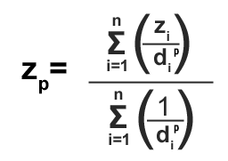
The sigma notation simply means that you are adding whatever number of points will be interpolated. Here we are simply summing the elevation values at each point for distance.

A smaller number in the denominator (more distance) has less effect on the interpolated (x_p) value. You’re also never going to have values above or below your maximum and minimum known values… So you better hope you have your highest or lowest points in your sample points!

Try plugging in different values. The math really isn’t so bad!

Try It Yourself

Given a set of known values such as elevation or noise, you now have the tools to estimate at points where you don’t know its value.

IDW uses spatial autocorrelation in its math. Closer values have more effect while farther away ones have less effect.

Specify the search distance or number of closest points. Set up a barrier. Choose a higher power setting for more localized peaks and troughs.

The Inverse Distance Weighting interpolation method is as flexible as they come. But it’s often the case that other interpolation techniques like kriging can help obtain a more robust model.