Kriging Interpolation – The Prediction Is Strong in this One

Sculpt a Legendary Prediction Model with Kriging

It’s time to sculpt a prediction model of the ages. The prediction is strong in kriging.

On your journey to creating a fine prediction surface, you’ll need to understand some key concepts before even getting into kriging.

What are these concepts?

Read below to get a step-by-step core knowledge of kriging.

Let’s start with some basics

To really understand kriging, you have to know what interpolation is. As with all interpolation, we’re predicting unknown values at other locations.

With an interpolation method like inverse distance weighting, you are making predictions without saying how certain you are.

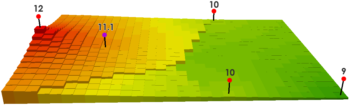
Here’s an example:

We predict the purple point, by taking an inverse weighted distance of the closest three input points (The values of 12, 10, and 10). Based on the distance, we calculate how far each input point is and get a value of 11.1.

((12/350) + (10/750) + (10/850)) / ((1/350) + (1/750) + (1/850)) = 11.1

This is exactly how deterministic interpolation works. Simply, it uses a predefined function and it is what it is.

But it doesn’t tell you how sure you are.

What is Kriging Interpolation?

If a weatherman makes a forecast saying it’s going to rain tomorrow, how sure are you that it’s going to rain?

In other words:

Instead of only saying here’s how much rainfall is at specific locations, kriging also tells you the probability of how much rainfall is at a specific location.

You use your input data to build a mathematical function with a semivariogram, create a prediction surface, and then validate your model with cross-validation.

Not only does geostatistics provide an optimal prediction surface, but it also delivers a measure of confidence in how likely that prediction will be true.

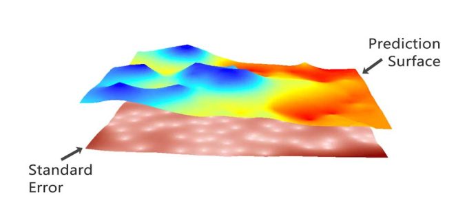
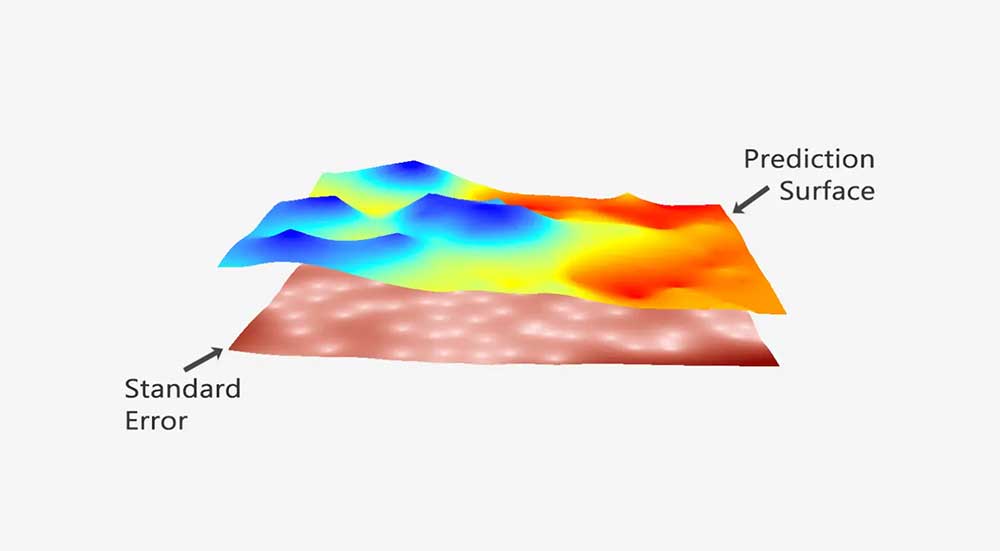
Meanwhile, kriging can generate prediction surfaces and surfaces that describe how well your model predicts:

PREDICTION: This surface directly predicts the values of the variable you are kriging.
ERROR OF PREDICTION: It depicts the standard error. You get a higher “standard of error” when there isn’t as much input data.
PROBABILITY: The probability surface highlights when it exceeds a threshold.
QUANTILE: This surface represents the best or worst-case scenarios as the 99th percentile.

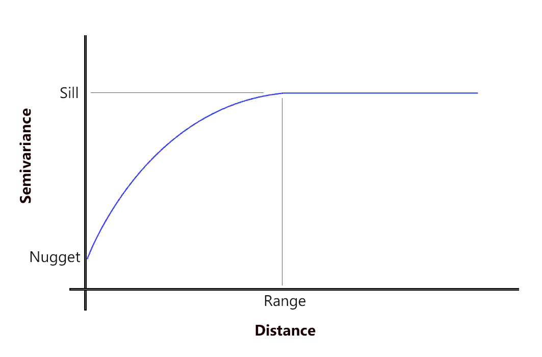
The Key to Kriging is the Semivariogram

Kriging relies on the semi-variogram. In simple terms, semivariograms quantify autocorrelation because they graph out the variance of all pairs of data according to distance.

Chances are that closer things are more related and have small semi-variance. While far things are less related and have a high semi-variance.

But at a certain distance (range), autocorrelation becomes independent. Where that variation levels off, it’s called (sill). This means there is no longer any spatial autocorrelation or relationship between the closeness of your data points. This concept is Tobler’s First Law of Geography.

Again, the purpose here is to fit a surface such as a polynomial that models the overall large-scale trend. Then, around that trend, we have variability with residuals where kriging comes in.

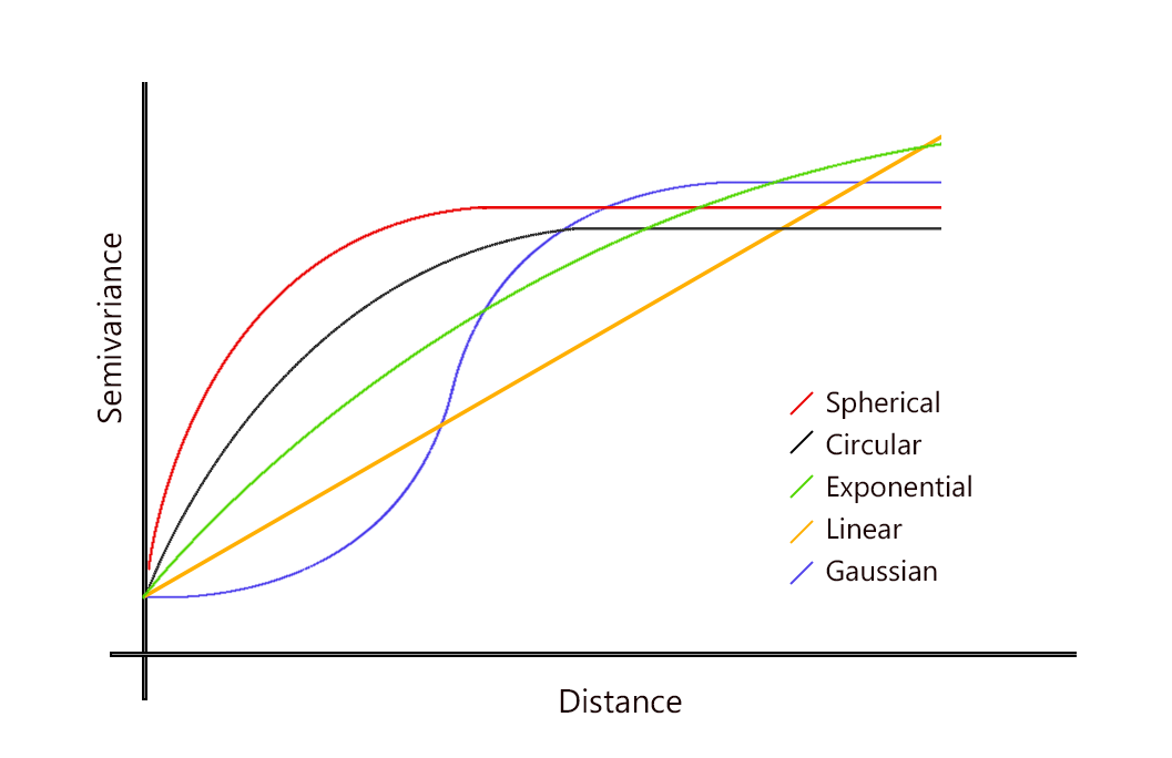
Based on your semi-variogram results, you can select a semivariogram that is spherical, circular, exponential, Gaussian, or linear. Alternatively, if you can make an intellectual justification for a mathematical model, then you pick that one.

Before You Even Begin, Check Your Data

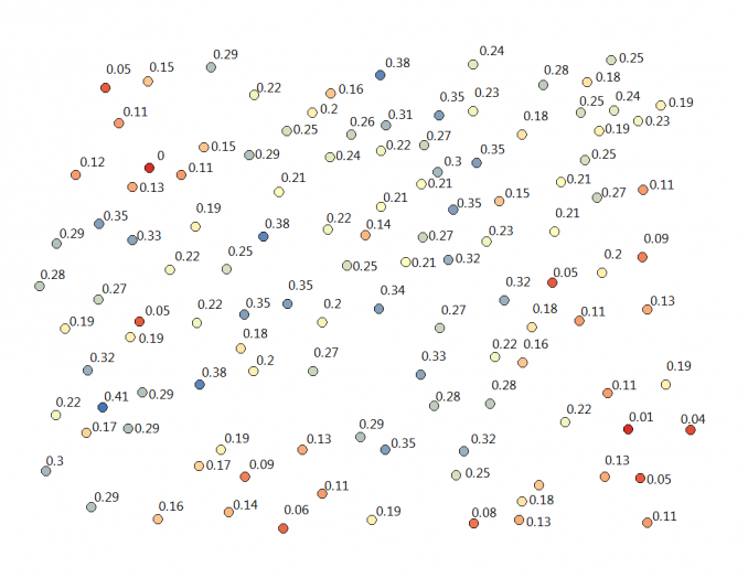
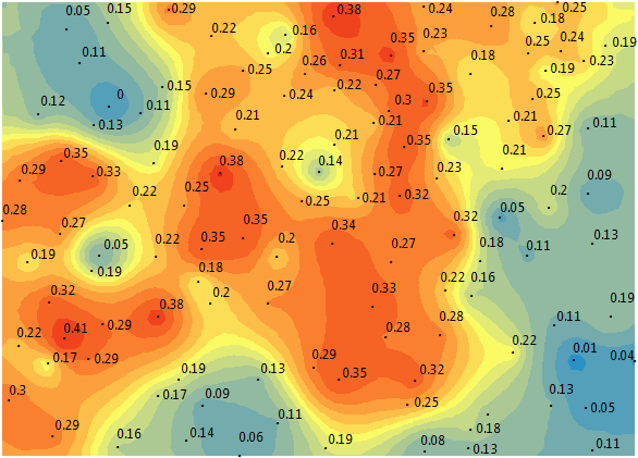
In our example, we use soil moisture samples taken in an agriculture field. Here is a visualization of our data points with soil moisture measurements.

Before you even start kriging, your data needs to fit these criteria before ordinary kriging.

Kriging is the optimal interpolation technique if your data meets certain criteria. But if they don’t meet those criteria, you can massage it or choose a different interpolation technique altogether.

• Your data needs to have a normal distribution
• The data needs to be stationary
• Your data cannot have any trends

The following steps are ways to check your data to see if they fit these criteria. First, we suggest plotting out your points and symbolizing them from low to high.

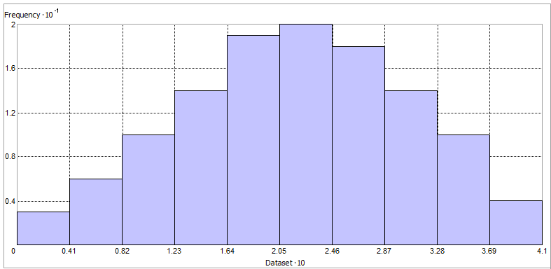
Assumption 1. Your data has a normal distribution

While we are not exploring the spatial properties in this test, we are only checking that the values are fairly normally distributed. In other words, do the values of your data fit a bell-curve shape?

One of the ways to explore this is by using a histogram. In ArcGIS, click Geostatistical Analysis > Explore Data > Histogram.

At this point, you can check the histogram for any outliers and how much it looks like a bell curve. In our case, it looks like it has a fairly good normal distribution.

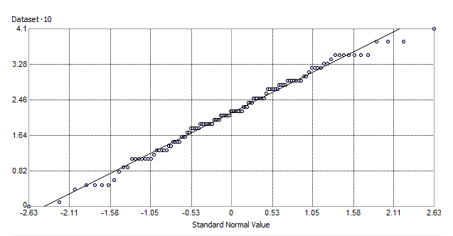
Alternatively, you can check your data with a Normal QQ Plot. A Normal QQ Plot compares how your data lines up with normally distributed data. If all points have a perfectly normal distribution, all your points would fall on the 45° line. In our case, the data follows a straight line.

What if your data doesn’t have a normal distribution?

In this case, you will have to apply a transformation such as Log or Arcsin until it becomes normal. Instead of selecting your own transformation, you can do a normal score transformation which pretty much does a lot of the work for you.

The normal score transformation is so powerful that it’s now the default method as simple kriging in ArcGIS. We explain this in more detail below.

Assumption 2. Your data is stationary

What does it mean that your data has to be stationary?

It means that local variation doesn’t change in different areas of the map. For example, 2 data points 5 meters apart in different locations should have similar differences in your measured value. The variance is fairly constant in different areas of the map. Kriging is not optimal for abrupt changes and breaklines.

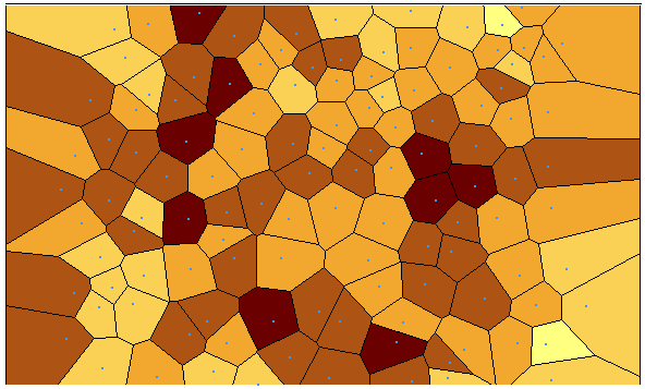
You can check your data’s stationarity with a Voronoi map symbolizing by entropy (variation between neighbors) or standard deviation and look for randomness. In ArcGIS, click Geostatistical Analysis > Explore Data > Voronoi Map.

READ MORE: What Is a Voronoi Diagram?

In our case, we do see some small amounts of clustering. Overall, for entropy and standard deviation, Voronoi maps show the data set is looking adequately stationary.

What do you do if your data isn’t stationary?

Empirical Bayesian Kriging (EBK) can help by treating local variance separately. Instead of variance being similar to a whole extent, EBK performs kriging as a separate underlying process in different areas. It still performs kriging, but it is done locally.

Assumption 3. Your data doesn’t have trends

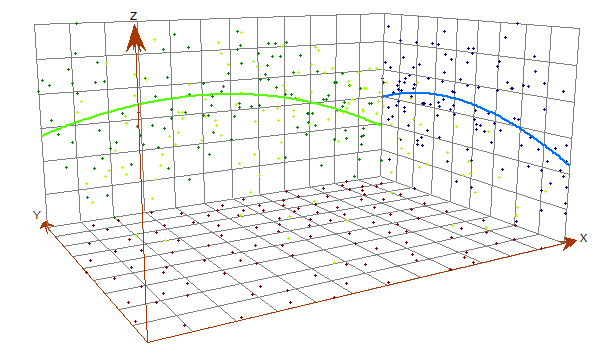
Trends are systematic changes in data across an entire study area. We can check the trend analysis with the ESDA tool. In ArcGIS, click Geostatistical Analysis > Explore Data > Trend Analysis.

The green line shows the trend in the east-west direction, and the blue line depicts the trend in the north-south direction. Generally, we have higher soil moisture values in the center. But there’s not enough of a trend in our data that it needs to be removed.

What if your data has systematic trends?

Although having large trends in your entire study area may be a reason to switch interpolation methods altogether, the trend removal tool can assist so the following analysis will not be influenced by that trend in your data.

Kriging Example in ArcGIS

After exploring your data for the above criteria, you can click Geostatistical Analysis > Geostatistical Wizard.

…And now the fun truly begins

(This is said with a load of sarcasm)

Step 1. Select Either Kriging/Co-Kriging

Now that you have the Geostatistical Wizard open, kriging is under the geostatistical methods. As mentioned earlier, this is because you build your optimal prediction surface with a semivariogram and can estimate a measure of confidence of how likely that prediction will be true.

Notice how if you select a single input, it’s simply kriging. But when you add a second variable, it suddenly becomes co-kriging.

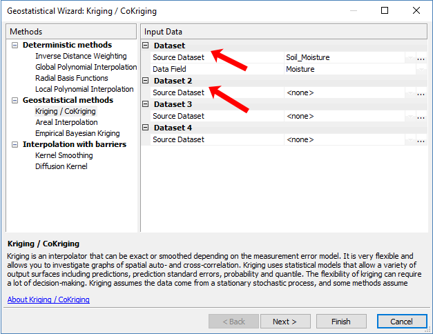
If you have 2 or more variables that are related to how precipitation changes in mountain areas, then you can add elevation data as a covariate to rainfall amounts. In this case, you can improve the prediction with secondary information.

Step 2. Choose the Kriging Type

Now, let’s take a step back for a second to understand what all the options mean. There’s quite a bit to absorb in this step.

Ordinary kriging was the default in ArcGIS 10.0. Now because of normal score transformation, simple kriging is the default. In particular, simple kriging uses a normal score transformation transforming your data into a standard normal distribution.

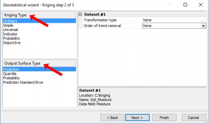
As mentioned earlier, this is one of the essential criteria to perform kriging. For basic users, your best option is taking the simple kriging approach. But other more complicated kriging types exist:

UNIVERSAL KRIGING combines trend surface analysis (drift) with ordinary kriging by accounting for trends
INDICATOR KRIGING carries through ordinary kriging with binary data (0 and 1) such as urban and non-urban cells.
PROBABILITY KRIGING uses binary data (similar to indicator kriging) and estimates unknown points for a series of cutoffs.

Lastly, you can manually set your transformation type and trend removal in this step. For example, if you want to change your transformation to log, this is when you can make this change.

Step 3. Model Data With a Semi-Variogram

In this example, we use ordinary kriging for demonstration purposes. The geostatistical wizard generates a semivariogram with blue crosses showing the average variation for each pair of points.

The lag size is the size of a distance class into which pairs of locations are grouped. As a rule of thumb, you can multiply the lag size by the number of lags for it to equal half of the largest distance among all points. If your points aren’t clustered, you can run the ‘Average Nearest Neighbor’ tool which tells you the average distance between points.

ArcMap has added the functionality to optimize all these parameters for you. When you click the optimize button, it will find the value for each parameter that results in the smallest root mean square error. That would be a lot of trial-and-error for the user to test each scenario. Ultimately, it’s usually best to go with the semivariogram model that the software thinks is best.

For our study area, here is what the semivariogram looks like:

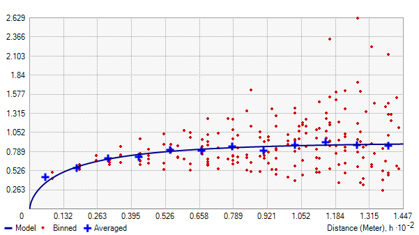
Remember that semi-variograms simply take 2 sample locations and call the distance between both points h.

On the x-axis, it plots distance (h) in lags, which are just grouped distances. Taking each set of 2 sample locations, it measures the variance between the response variable (water content in soil) and plots it out on the y-axis.

Step 4. Map the Model with Kriging Weight

After you are satisfied with your fitted semi-variogram, the wizard gives a preview surface with even more parameters to customize the output. What kriging does is predict responses at each location using a weighted average with nearest neighbors. But first, you have to set the number of points (maximum and minimum) to use in your search radius.

Despite so much talk on how important semivariograms matter in kriging, this step influences the output of your map immensely. If you change any of these parameters, it can really alter the look and feel of the surface.

If you select one of the slice sector types, this ensures that there will be points included to estimate in each one of those slices. For example, if you use a four-slice pie and set your neighbors to 5, then each slice will use 5 points (a total of 20) for local estimates.

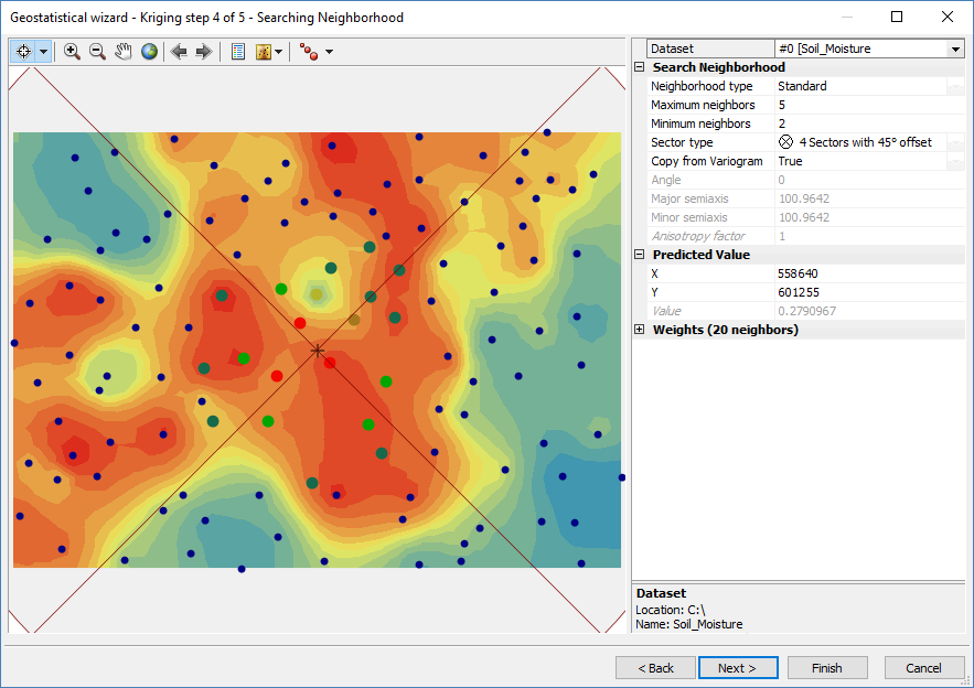
As there is no perfect set formula, the key is to pan around and check predicted values for how you feel the output should look.

Step 5. Check Cross-validation Results

The cross-validation step for kriging takes one of your input data points and throws it out of the data set. Using all of the remaining points, it runs the prediction back to that location. Again, you know what the true value is, this process uses all remaining to predict that value.

Cross-validation iterates through all of your input points until it’s complete. Then, it creates this summary table of residuals comparing actual versus your model’s predicted values. What this table shows is how robust your model really is.

So how close are true values to predicted values? In other words, how well does your model fit the data? To put this all in perspective, check your root-mean-square standardized, as it should be close to 1. In addition, the root mean square error should be as small as possible.

The Dynamic Geostatistical Layer

Because the output is a geostatistical layer, it’s dynamic, meaning you can change its output type as prediction, errors of prediction, probability, or quantile. Or you can even go back into the geostatistical layer and change the parameters if you don’t like the optimized output.

There is a science and art to kriging.

It’s not only how you pick your model from a semivariogram, but also how you set up the number of bins and other settings. This is the art of kriging.

When you represent your kriging surface, such as choosing the number of intervals, it can give a different impression of the results. While more classes give more detail, the data classification method (such as quantile or equal interval) arranges your data differently.

The Prediction Is Strong in Kriging

Spatial prediction involves some component of randomness. This is crucial with geostatistics when you’re making inferences on a data set.

Your kriging weights are estimated from the variogram. More specifically, it’s derived from the model you choose. The quality of the estimated surface is reflected in the quality of the weights. You want weights that give an unbiased prediction and the smallest variance.

In other words, kriging finds the spatial pattern. It then predicts unknown values based on that spatial pattern. With these predictions, kriging generates a measure of error or uncertainty. This means that you can estimate confidence in the prediction surface they are true not because of random chance.

Not only do you customize your mathematical function to build one, but you also use the power of statistical analysis – namely the semivariogram.

Kriging is a geostatistics method that predicts the value in a geographic area given a set of measurements. It’s used in mining, soil, geology, and environmental science.

No single cookie-cutter methodology works for everyone. As it relates to your data, only you can decide what those settings are and how best to generate a prediction surface.