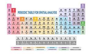
The Periodic Table for Spatial Analysis
Introducing: The Periodic Table for Spatial Analysis
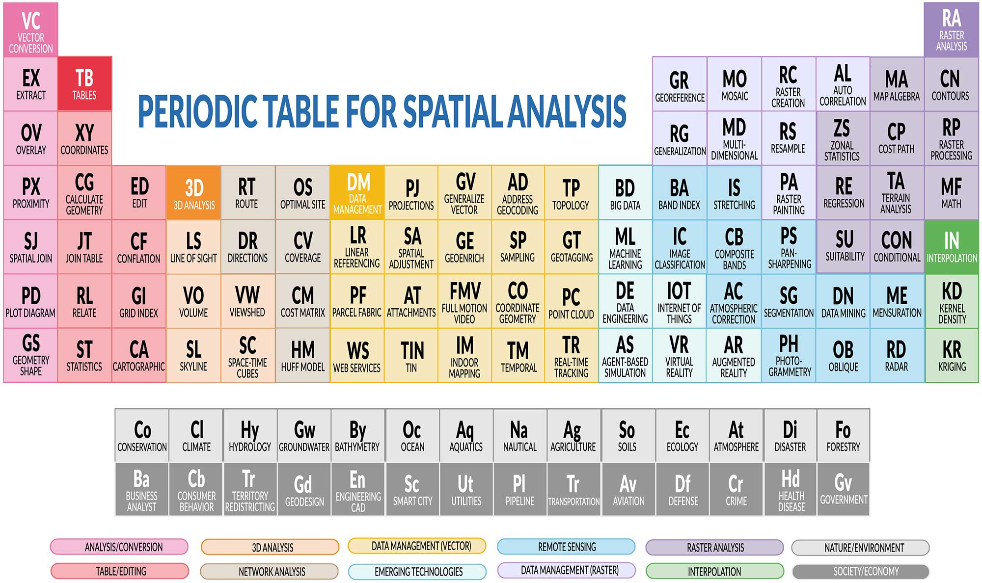
Each element in the Periodic Table for Spatial Analysis contains a set of spatial analysis tools. We’ve grouped common tools by color with vector analysis tools on the left and raster analysis on the right.
Vector Analysis/Conversion
1. Vector Conversion [VC] – Converts file formats for points, lines, and polygons and alters data models from vector to raster or vice versa. (Feature to raster, rasterization vs vectorization)
2. Extract [EX] – Creates a subset of features by clipping, selecting, and splitting vector features. (Clip, select, and split)
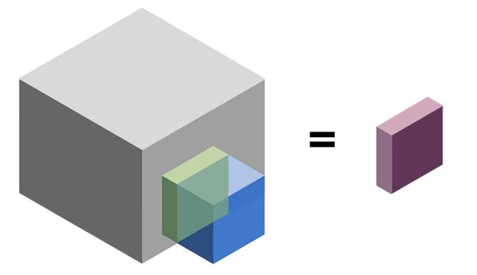
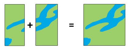
3. Overlay [OV] – Overlays 2 or more vector layers and outputs layers based on overlapping features. (Intersect, union, erase tool)
4. Proximity [PX] – Generates output based on distances or proximity functions. (Buffer, Voronoi diagrams, and near functions)
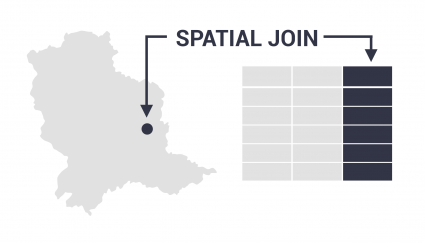
5. Spatial Join [SJ] – Joins attributes from a separate layer based on distance or spatial relationship. (1-M Spatial join “Contains”, 1-1 Touches)
6. Plot Diagrams [PD] – Builds a graph or diagram based on a set of attributes and geographical locations. (Scatter plot, histograms, bar plots)
7. Geometry Shape [GS] – Computes the geometric shape of an object. (Compactness, perimeter/area ratio, rectangular fit).
Tables
8. Table Tools [TB] – Performs table functions for storing attribute data (Add field, create domains, reorder fields)
9. Add XY Coordinates [XY] – Converts a table of XY coordinates (latitude/longitude) into a layer with a defined coordinate system. (Add lat/long coordinates)
10. Calculate Geometry [CG] – Computes the length of the geometric measurements in the attribute table of vector features. (Calculate length/area)
11. Join Table [JT] – Appends the attribute columns from one table into another table based on matching record keys. (1:1, 1:M, M:N)
12. Relate [RL] – Generates a temporary table that displays matching records that associate with one or more matching records. (Relate vs Join)
13. Statistics [ST] – Calculates statistics based on a numerical field in a table. (RMSE, MAE, sum, mean, count, standard deviation).
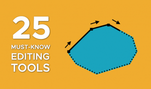
Editing/Cartography
14. Editing [ED] – Performs an editing function using the vertices and geometry in one or more layers. (Editing tools, densify, trim, snap, and extend)
15. Conflation [CF] – Resolves conflicts between two layers that display the same features with mismatching geometries. (Edge-matching, rubber sheeting, conflation)
16. Grid Index [GI] – Produces a set of consecutive rectangular map sheets that follow a linear feature for mapbook production. (Strip Map, fishnet, tessellation, QGIS Atlas, data driven pages)
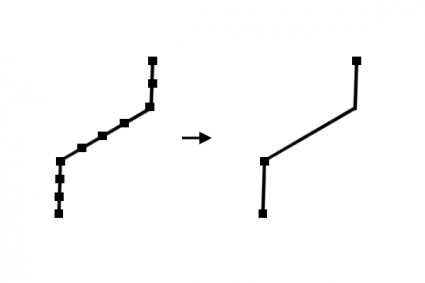
17. Cartographic [CA] – Enhances or generalizes features in a dataset for cartographic display and aesthetic quality. (Smooth, simplify, aggregate).
3D Analysis
18. 3D Analysis [3D] – Performs an overlay or proximity analysis with 3D features. (3D analysis buffer, intersect, or union)
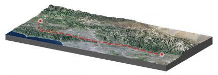
19. Line of Sight Visibility [LS] – Identifies obstruction and non-obstruction sections of a straight line from an observer. (Line of sight)
20. Volume [VS] – Calculates the amount of space above, below, within, or for the purpose of removing or adding material. (Cut/fill)
21. Viewshed [VW] – Determines locations visible to an observer in all directions with the output as a visibility raster.
22. Skyline [SL] – Displays visible and obstructed shadowed areas similar to a 3D fan pointing from an observer’s point of view.
23. Space-time Cubes [SC] – Builds temporal and 3D cubes representing slices of time in a geographic area. (Space-time cubes)
Network Analysis
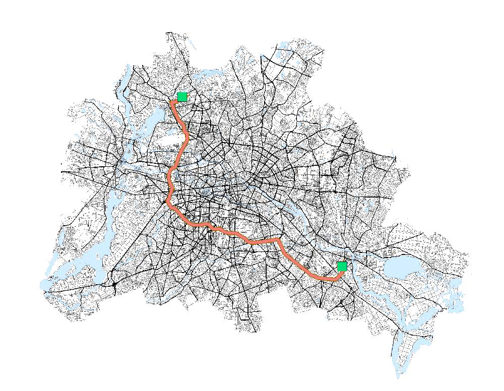
24. Route [RT] – Finds the optimal route using a set of points and a network dataset. (Network analysis fastest route, find nearest, or shortest distance)
25. Directions [DR] – Lists the turns, streets, and directions from an origin to a destination point using a network dataset.
26. Optimal Site [OS] – Selects optimal sites from existing facilities, competing stores, and available demand. (Location-allocation)
27. Coverage [CV] – Computes the coverage or accessibility that a facility can be reached for a given distance, time, and network dataset. (Service area)
28. OD Cost Matrix [CM] – Measures the least cost path from multiple origin points to multiple destination points.
29. Huff Model [HM] – Predicts the probability that consumers will patron retail stores using store size, distance, and census tract population. (Huff gravity model)
Data Management
30. Data Management [DM] – Manages layers with a set of tools to develop, alter, and maintain layers (Merge, append, data compare)
31. Projections [PJ] – Assigns a coordinate reference system for a layer. (Project, define projection)
32. Generalize Vector [GV] – Combines adjacent features or slivers based on common attribute values or shared borders. (Dissolve and eliminate)
33. Address Geocoding (AD) – Translates addresses into geographic locations with latitude and longitude coordinates. (Geocode, reverse geocode)
34. Topology [TP] – Fixes and catches editing errors such as overshoots, undershoots, slivers, overlaps, and gaps. (Topology rules)
35. Linear Referencing [LR] – Stores relative positions on a line feature represented by m-values for point/line events. (Linear referencing systems)
36. Spatial Adjustment [SA] – Aligns and transforms a vector layer that has been displaced, rotated, or distorted like georeferencing for vectors. (Vector bender, displacement links)
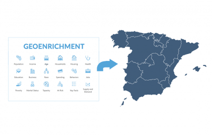
37. GeoEnrich [GE] – Ameliorates existing data with value-added information such as demographic, education, or income attributes. (GeoEnrichment)
38. Sampling [SP] – Creates a subset of data for sampling at set intervals or randomly. (Regular points, random points in extent)
39. Geotagging [GT] – Assigns geographic coordinates to digital photos through GPS without georeferencing. (Geotagging)
40. Parcel Fabric [PF] – Constructs cadastral specific to managing parcel fabric. (Cadastral divisions, split polygon)
41. Attachments [AT] – Builds attachments to store photos internally as a table relationship.
42. Full Motion Video [FMV] – Geo-enables video with the footprints coordinated on a map. (Full motion video)
43. COGO [CO] – Captures coordinates, bearings, and distances from transverse land survey measurements. (COGO – Coordinate Geometry)
44. Point Cloud [PC] – Manages LAS files with a set of tools to maintain, alter, and interpolate point clouds.
45. Web Service [WS] – Deploys or imports features from a layer as a web feature/mapping service. (Web feature service, GeoRSS)
46. TIN [TIN] – Creates a triangular irregular network for depicting three-dimensional terrain surfaces. (TIN mesh creation)
47. Indoor Mapping [IM] – Incorporates indoor floor plans with digital formats like BIM, Revit, and CAD. (Indoor mapping)
48. Temporal [TM] – Adds time properties to layers with the date and/or time (Convert time zone, update time field, temporal animation)
49. Real-time Tracking [TR] – Streams real-time movement of objects or change in status over time. (GeoEvent server, geofencing, make tracking layer)
Emerging Technology

50. Big Data [BD] – Analyzes and extracts data from datasets too large and complex with geographic locations. (GeoAnalytics Desktop Tools)
51. Machine Learning [ML] – Uses neural networks for classification, prediction, and segmentation through training and labeling. (Deep learning toolset, machine learning)
52. Data Engineering [DE] – Validates, cleans, and maintains spatial data into a usable form for analysis.
53. IoT [IOT] – Analyzes real-time data feeds and sensors from the Internet of Things (IoT) platform. (ArcGIS Velocity)
54. Agent-based Simulation and Modeling [AS] – Simulate scenarios and the emergence of phenomena through individual interactions in geographic space. (Multi-agent modeling environment)
55. Virtual Reality [VR] – Replaces the field of vision through headsets in a spatial environment.
56. Augmented Reality [AR] – Enhances 3D features on your phone’s display to interact spatially with the outside world. (Augmented reality)


Raster Data Management
57. Georeferencing [GR] – Stretches, scales, rotates, and skews raster images to better relate to geographic space. (Georeferencing)
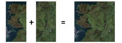
58. Mosaic [MO] – Combines multiple raster images into a seamless, composite raster image. (Mosaic)
59. Raster Creation [RC] – Generates a raster for a given extent at a specific cell size. (Create a random raster, create a constant raster)
60. Spatial Autocorrelation [AL] – Measures how dispersed or clustered cells are located in a raster. (Moran’s I)
61. Generalization [RG] – Cleans raster data by generalizing, smoothing, and altering cells. (Nibble, shrink, expand)
62. Multidimensional [MD] – Provides an interface for array-oriented data for storing multidimensional variables. (NetCDF)
63. Resample [RS] – Updates the cell size for converting raster images. (Raster resample: Nearest neighbor, bilinear, and cubic convolution)
64. Raster Painting [PA] – Draws and erases raster cells with a set of brush, fill, and erase tools.
Raster Analysis
65. Raster Analysis [RA] – Performs raster analysis functions for a raster grid dataset. (Analyze patterns)
66. Map Algebra [MA] – Applies math-like operations in local, zonal, focal, and global configurations. (Map algebra)
67. Contours [CN] – Produces lines of constant elevation to represent the topography of the landscape. (Contours)
68. Zonal Statistics [ZS] – Generates statistics for defined zones of a raster surface. (Zonal statistics – mean, sum, and majority)
69. Cost Path [CP] – Finds the most cost-effective path, from a start point to a destination, which accumulates the least amount of cost. (Least cost path)
70. Raster Processing [RP] – Creates a subset of features by clipping, selecting, and splitting raster grids. (Raster clip, split raster)
71. Spatial Regression [RE] – Generates a prediction surface based on explanatory variables. (Ordinary least squares regression, spatial regression)
72. Terrain Analysis [TA] – Calculates the characteristics of the terrain from an input raster. (Slope, morphometry, TPI, and roughness)
73. Math Function [MF] – Executes a math function to update the numerical value on a cell-by-cell basis. (Arithmetic, power, exponential, and logarithmic)
74. Suitability [SU] – Overlays raster surfaces based on criteria to analyze suitability. (Fuzzy logic weighted sum)
75. Conditional [CON] – Performs a conditional statement on a raster that generates a binary output. (Greater than, equal to)

Remote Sensing
76. Band Index [BA] – Converts a set of imagery bands by leveraging the inherent wavelength properties. (NDVI, tasseled cap, wetness index)
77. Image Stretching [IS] – Arranges the display of an image by adjusting brightness, contrast, and gamma properties.
78. Image Classification [IC] – Assigns land cover classes to imagery pixels based on their spectral properties. (Supervised/unsupervised classification)
79. Composite Bands [CB] – Combines single-band rasters into a composite raster for true color or false color display. (Composite bands)
80. Pansharpening [PS] – Enhances spatial cell resolution by leveraging the panchromatic band.
81. Atmosphere Correction [AC] – Corrects remote sensing imagery through scattering inherent in the atmosphere. (Dark object subtraction, radiative transfer models, atmosphere correction)
82. Segmentation [SG] – Grouping similar pixels from an image into vector objects to recognize objects and features. (Segment mean shift, object-based image analysis)
83. Data Mining [DN] – Eliminates redundant data from variables that are highly correlated, aggregating essential information. (Principal component analysis)
84. Mensuration [ME] – Measures the geometry of two and three-dimensional features in an image. (Angles, height, perimeter, volume)
85. Photogrammetry [PH] – Performs stereographic parallax from two or more vantage points of the same object to measure relief displacement. (Photogrammetry)
86. Oblique [OB] – Collects images at an angle as opposed to a top-down orthographic perspective.
87. Radar [RD] – Measures the backscatter of a sent microwave pulses to Earth whether it’s specular, diffuse, or double-bounce reflection. (Synthetic aperture radar)
Interpolation
88. Interpolation [IP] – Estimates unknown values using sampled locations by creating a prediction surface. (IDW, spline, trend)
89. Kriging [KR] – Generates a probability and prediction surface by building a mathematical function through a semi-variogram. (Kriging and semi-variograms, and geostatistics)
90. Kernel Density [KD] – Calculates hot and cold spots by applying a density-per-unit function (Heat map)
Conclusion: The Periodic Table for Spatial Analysis
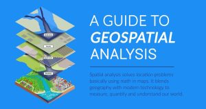
Spatial analysis may seem like alchemy to the inexperienced. But there is a science to it. By using spatial analysis, we can find patterns, quantify area, and predict outcomes with geography being the common link of it all.


This is genius. For GIS development or spatial data systems, this is a good guide. Good luck.
Awesome, as a newcomer to the field, this is very helpful and enjoyable.. but where can I get a printable version of this? :=)
Hi Gregor. Please feel to download/print and use for your personal use.
Excellent work; hats off to you.
Nice, insightful contents on geospatial
Great Achievement!
This is an amazing work
Great!
This is for GIS bible.
This is a great 👍🏿 one sir. Thank you
I appreciate your effort which shows how deep you have been gone in spatial science.
Thanks for sharing us!
Excellent work.
Amazing stuff, very nicely presented. Appreciate you sharing this.
question <- "is spatial statistics element of spatial analysis?"
if (question == TRUE){
return("the table is missing the statistical component. Can it be added?"
} else {
return("Excellent table. Great Job")
}
A fantastic and useful visual tools for Spatial Analysis lovers like me… Thanks and great job!
Great Stuff. Provides an insight to what you dont know.
This is really makes me proud of being a Geospatial scientist
I like this portrayal but it’s missing the Quality Control element………….
Wonderful! I will print out
This is really good 👍
Amazing creativity! I’ll show this to everyone I can.
Thanks for creating this visual depiction of basic and traditional routines for spatial data processing and analysis. It’s a great tool to help illustrate and explain the various academic disciplines that come together to form a well-rounded professional in this field.
Top notch creativity!
I’ll spread the word to my students
Great information to share to the mass.
This is amazing, thanks so much for compiling!! Can’t wait to use this in ALL my GIS classes.
Please elaborate more on GIS, remote sensing, spatial analysis, and GPS for beginners
Very clever – thank you all! I will tell others about this and use it in my own courses and in teaching.
–Joseph Kerski
Grateful.
Very clear and super explanatory document.
This is a great composition of the ideals of my beloved field. I am a proud professional geographer whose tools are enshrined in computational geography – GIS, Remote Sensing, and Spatial Analysis. I will ensure that I commit this to memory to teach my students and mentees.