What Is Geographically Weighted Regression (GWR)?

Geographically Weighted Regression (GWR) is a spatial statistical technique that models the relationship between a dependent variable and independent variables while allowing for spatial variation in the model parameters, making it sensitive to local geographic variations.
What is a Geographically Weighted Regression Model?
The tech-savvy GIS detective loves spatial regression because it’s used to model spatial relationships. Regression models investigate what variables explain their location.
For example: If you have crime locations in a city, you can use spatial regression to understand the factors behind patterns of crime. We can use spatial regression to understand what variables (income, education, and more) explain crime locations.
A spatial regression model can then be used for decision-making. For example, it can answer where are suitable locations for police stations. Spatial regression models are also used to predict future crime locations and even in other cities.
Let’s understand some of the terminologies in regression models.
- Dependent variable (Y): What you are trying to predict. (Location of crimes)
- Independent variable (X): Explanatory variables that explain the dependent variable. (Income, education, etc)
- Beta-coefficient: Weights that reflect the relationship between the explanatory and dependent variables.
- Residual: The value not explained by the model
Geographically Weighted Regression Formula:
y = β0 + (β1 × x1) + (β2 × x2) + … + (βn × xn) + Ε
Spatial Regression Analysis in ArcGIS
Let’s put the ArcGIS regression tools in action by building a habitat suitability index (HSI) – also known as a Resource Selection Function (RSF). With 308 GPS locations of marsh deer, we investigate the relationship between marsh deer and their landscape.
Important to note: This is a hypothetical scenario with made-up data.
We answer questions like:
- Which resources do marsh deer select or avoid?
- What are some of the factors that contribute to the location of marsh deer?

Habitat Suitability Index (HSI)
Habitat Suitability Index (HSI): An HSI is a numerical index that represents the capacity of a given habitat to support a selected species
Why create an HSI?
A land resource manager uses HSI to make better decisions on the landscape. If an HSI shows marsh deer prefer wetland habitat types, a land resource manager can preserve these types of habitat.
A land resource manager can prohibit the development of infrastructure because an HSI shows the capacity of a given habitat to support marsh deer. We can extrapolate HSI to predict marsh deer in other locations.
Explanatory Variables
What are the explanatory variables for marsh deer? This may be the most difficult part of regression modeling. We need to investigate potential habitat types for Marsh deer. This is where expert advice comes in handy. Here’s what we found:
“Marsh deer are found in marshy habitats such as floodplains, grasslands, and moist forests, preferring areas with a good amount of cover for protection, such as reed beds or where grass stands are high. This species is predominantly found close to permanent sources of water.”
Based on the literature, Marsh deer select natural vegetation and water. But are there any land features that potentially disturb Marsh deer? We explore these independent variables using our spatial regression analysis.
Independent and Dependent Variables
Our study area is characterized by natural vegetation and open water. A road cuts through cells A6-F6 which may act as a potential disturbance. Campgrounds are also present in cells B3, C7, and D7.
Marsh Deer Distribution and Campgrounds
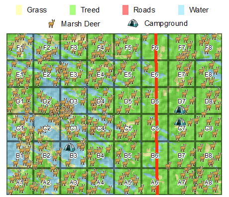
Each dot represents the GPS position of the marsh deer. Visually, there appear to be fewer marsh deer near roads and campgrounds. Another observation is that marsh deer appear denser in cells D2 and D3 where wetlands are present.
Hotspot Analysis
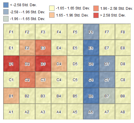
This hotspot map confirms fewer deer close to roads to a degree of less than -2 standard deviations from the mean. Marsh deer are denser near cells D2. Other than these two low hotspots, there don’t appear to be any more spatial patterns in the study area.
- Why are there so many deer in these hot spots?
- What are some of the factors that contribute to these hot spots?
We can answer these types of questions using regression analysis. Let’s use spatial regression to model spatial relationships between marsh deer and land features.
Ordinary Least Square (OLS) Regression
The first step is to group the independent and dependent variables per grid cell. We cannot look at the Marsh deer locations as points. The table must have the number of deers, campgrounds, and wetlands for each grid cell. The table below is an example of a pre-processed table using OLS.
| Cell | Deer | Road | Water | Camp |
|---|---|---|---|---|
| A1 | 9 | 0 | 30 | 0 |
| A2 | 7 | 0 | 25 | 0 |
| A3 | 9 | 0 | 15 | 0 |
We will use the “Ordinary Least Squares Regression” tool in the “Modelling Spatial Relationships” toolkit.
Ordinary Least Square Regression Model:
Input Feature Class: Grid cells with aggregated data
Unique ID: A unique ID field (ex, 1, 2, 3…)
Output Feature Class: Path and name of the output
Dependent Variable: Deer count
Explanatory Variables: Campgrounds, roads, and water
Output report file: Generates a report file.
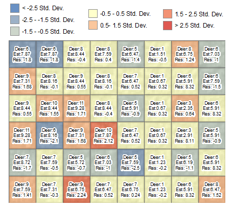
After running the OLS tool, the residuals of the prediction model will be added to your display. The residuals are essentially the error in the model.
Let’s take a closer look at what a residual actually is before moving forward. If we look at cell A1 (bottom left), there were 9 deer found in this grid cell. The OLS model built weights based on the number of trees, wetlands, grass, roads, and campgrounds in the cell. These weights are the beta-coefficient values.
When we plugged the weights into the regression formula, there was an estimated 6.98 deer in cell A1. When you subtract 6.98 from 9, we get a residual of 2.01. In other words, the model underpredicts the actual value by 2.01.
Ordinary Least Squares Regression Residuals Values:
| Variable | Beta-coefficient | p < 0.05 | VIF |
| Intercept | β0 = 5.916744 | 0.0000001* | —– |
| Roads | β1 = -0.524393 | 0.0000001* | 1.150233 |
| Water | β2 = 0.056088 | 0.0000001* | 1.139367 |
| Camp | β3 = -3.558805 | 0.0000001* | 1.010354 |
You can interpret the low negative beta-coefficient of campgrounds (-3.56) as areas where marsh deer avoid. Roads as well had a negative value of -0.52, meaning deer do not select these grids. Marsh deer prefer wetlands as a suitable habitat. This model confirms this belief.
We can manually plug the beta-coefficient model into the regression model. The result is the predicted value. In our case, it is the predicted number of deer in the grid cell.
y = β0 + (β1 × x1) + (β2 × x2) + … + (βn × xn) + Ε
A1 = 5.916744 + (-0.524393 × 0) + (0.056088 × 30) + (-3.558805 × 0)
A1 = 7.59
This OLS model achieves an adjusted R-squared value of 0.795. With these 3 factors, we can explain 79.5% of the variation that’s occurring.
What is the model missing? Known predators, forest age, wetland type.
Variance Inflation Factor (VIF):
Another statistic of interest is the Variance Inflation Factor (VIF). If the VIF > 7.5, this indicates redundancy among explanatory variables. Our HSI model satisfied these criteria with VIF < 2.0.
Probability and Robust Probability:
An asterisk (*) indicates that the coefficient is statistically significant (p < 0.05). The Marsh deer HSI had p-values < 0.0001 meaning the coefficients are statistically significant.
Jarque-Bera Statistic:
When this test is statistically significant (p < 0.05) model predictions are biased (the residuals are not normally distributed). The Jarque-Bera Statistic score was 0.721. When the OLS regression models tools give the WARNING 000851 at the end of the report, this means that the Spatial Autocorrelation (Moran’s I) Tool should be processed to ensure residuals are not spatially autocorrelated.
Moran’s I Spatial Autocorrelation
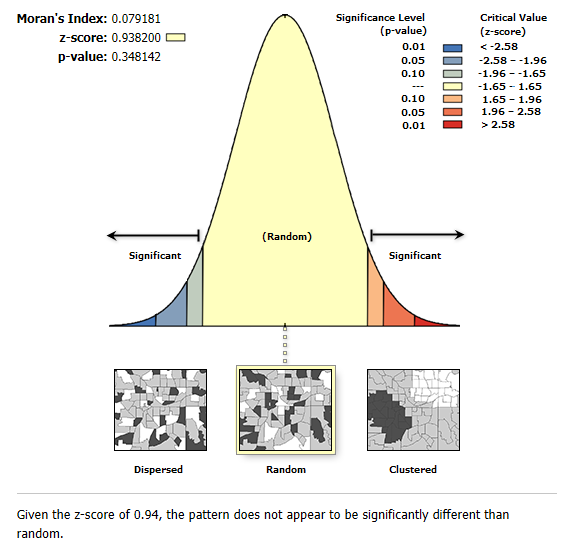
The spatial autocorrelation will tell us if the under/over predictions are random. No model can predict perfectly and will always over and underpredict. Spatial autocorrelation investigates if the OLS model is randomly distributed.
Moran’s I Spatial Autocorrelation:
Input Feature Class: OLS output
Input Field: Standard Residual (StdResid)
Generate Report: YES
When you click OK, the tool generates a report. Double-click the report, and ensure that the results are random.
Geographically Weighted Regression

We built a spatial relationship between Marsh deer, campgrounds, roads, and wetlands using the spatial regression tool. Regression tools investigated the relationship between these factors and generated weights for each variable.
These weights were plugged into the regression formula to calculate and predict the number of deer. The variance inflation factor, z-scores, Jarque-Bera, and Moran’s I ensured robustness and statistical significance in the spatial regression model.
The regression model shows how Marsh deer select wetlands as a suitable habitat. It also shows that Marsh deer tend to avoid campgrounds and roads.
This is useful to land resource managers to potentially restrict the development of campgrounds and roads to conserve this type of deer. The regression model can also predict Marsh deer in other areas.