Principal Component Analysis (PCA) in GIS
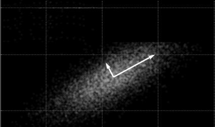
PCA. You’ve probably seen this acronym before. PCA stands for “Principal Component Analysis“.
But what is it? And how do we use it in GIS and remote sensing?
Sometimes, variables are highly correlated in such a way that it would be duplicate information found in another variable. The principal component analysis identifies duplicate data over several datasets. Then, PCA aggregates only essential information into groups called “principal components“.
The power of PCA is that it creates a new dataset with only the essential information. The bottom line is that you reduce redundancy when using PCA.
What is Principal Component Analysis in GIS?
So the principal component analysis catches redundancy between data sets.
But what about elevation, slope, and hillshade data? Is there redundancy in these three data sets? If so, how much?
Today, let’s explore how to run a PCA analysis with elevation, hillshade, and slope bands using ArcGIS Desktop.
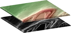
Step 1. Run the “Composite Bands” tool
The “Composite Bands” tool combines the elevation, hillshade, and slope rasters into a single 3-band raster. Use the following rasters as inputs:
- ELEVATION: Band 1
- HILLSHADE:: Band 2
- SLOPE: Band 3
Output the new raster as Composite
Step 2. Execute the “Principal Components” tool
Using the spatial analyst extension in ArcGIS, execute the “Principal Components” tool with the following criteria:
- INPUT RASTER: Composite
- OUTPUT RASTER: PCA
- NUMBER OF PRINCIPAL COMPONENTS: 3
- OUTPUT DATA FILE: PrincipalComponents.txt
The result will be a 3-channel PCA composite and a data file showing the amount of redundancy.
Step 3. Analyze the Principal Components Table
The “Percent of Eigenvalues” shows how much each principal component accounts for.
| PC Layer | EigenValue | Percent of EigenValues | Accumulative of Eigen Values |
|---|---|---|---|
| 1 | 699.9 | 67.1 | 67.1 |
| 2 | 323.6 | 31 | 98.1 |
| 3 | 19.5 | 1.9 | 100 |
This table shows that the first component accounts for 67.1% of the covariance.
When you add the second channel, it accounts for 98.1% of the covariance. The third component does not give much extra information (1.9%) and is slightly redundant with principal components 1 and 2.
How to use PCA in remote sensing?
Running a principal component analysis on three bands was useful because we found the third component did not add much information.
What about a 10-band multispectral image? Or even 100 or 200 bands (hyperspectral imagery)?
This is where PCA is really useful – multispectral and hyperspectral analysis.
For example, if most of the variance (eigenvalue) is found in principal components one, two, and three, it’s only necessary to use these three principal components. For land cover classification, it is much easier to use three bands compared to all 10 bands.
In summary, PCA identifies duplicate data over multiple channels, reduces redundancy, and speeds up the processing time. This is key for principal component analysis image processing.
What’s Next?
Where you’re working with highly correlated variables, you can run a principal component analysis to see which ones are redundant.
If you’ve tested this principal component analysis guide, try to master these other spatial statistics guides:







Can I use PCA techniques for assigning weights for several thematic layers in ArcGIS?
Hello everyone
I want to run PCA for lidar point cloud. how can I run it?
I keep getting a syntax error whenever I run pca on ArcMap. I even tried changing the output name to less than 10 characters and it still doesn’t work. Any suggestions?
I would rather not skip it, even if it doesn’t fit the purpose of your study. The general rule in PCA is the more the better.
Should I exclude Landsat 8-OLI Band#1 (Aerosol Band) from the composite image containing all multi-spectral bands.