Spatial Autocorrelation and Moran’s I in GIS

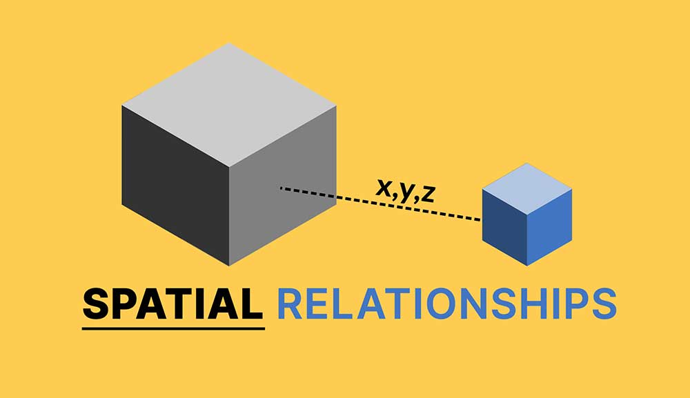
Spatial autocorrelation in GIS helps understand the degree to which one object is similar to other nearby objects.
Moran’s I (Index) measures spatial autocorrelation. Geographer Waldo R. Tobler stated in the first law of geography:
“Everything is related to everything else, but near things are more related than distant things.”
Spatial autocorrelation measures how close objects are in comparison with other close objects. Moran’s I can be classified as positive, negative, and with no spatial auto-correlation.
DEFINITION:
Spatial autocorrelation measures how similar or dissimilar values are at nearby locations. In other words, it measures whether things that are close together are also alike in value.
Why is Spatial Autocorrelation Important?
One of the main reasons why spatial auto-correlation is important is because statistics rely on observations being independent of one another. If autocorrelation exists in a map, then this violates the fact that observations are independent of one another.
Another potential application is analyzing clusters and dispersion of ecology and disease.
These trends can be better understood using spatial autocorrelation analysis.
Positive Spatial Autocorrelation Example
Positive spatial autocorrelation occurs when Moran’s I is close to +1. This means values cluster together. For example, elevation datasets have similar elevation values close to each other.
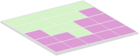
There is clustering in the land cover image above. This clustered pattern generates a Moran’s I of 0.60. The z-score of 4.95 indicates there is a less than 1% likelihood that this clustered pattern could be the result of a random choice.
Negative Spatial Autocorrelation Example
Negative spatial auto-correlation occurs when Moran’s I is near -1. A checkerboard is an example where Moran’s I is -1 because dissimilar values are next to each other. A value of 0 for Moran’s I typically indicates no autocorrelation.
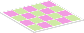
Using the spatial autocorrelation tool in ArcGIS, the checkerboard pattern generates a Moran’s index of -1.00 with a z-score of -7.59.
(Remember that the z-score indicates the statistical significance given the number of features in the dataset).
This checkerboard pattern has a less than 1% likelihood that it is the result of a random choice. If you want to test this statistical technique, try GeoDa software for this and more.
What’s Next: Spatial Dependency
Spatial autocorrelation indicates if there is clustering or dispersion in a map. While a positive Moran’s I hints that data is clustered, a negative Moran’s I implies data is dispersed.
If you’ve tested this spatial autocorrelation guide, try to master spatial statistics widely used statistics in GIS:


I don’t think you need spatial dependence analysis on this. Just carry out a survey. Ask questions using questionnaires or interview where they live, how close they are to railroad. Administer them to the people close to railway, ask of health challenges they have. Cancer should be one of the options to pick
I want to know that can I apply spatial auto correlation Moran’s I in identifying the location patterns of schools in a region. Whether the location patterns of the schools are clustered, dispersed, or random.
Thank you for these good info
I have three different configurations of points in my study area. Also I have 5 different variables (altitude, slope, …). My purpose is to select one of these point sets with least autocorrelation in the modeling process.
My question is that I must calculate Moran’s I for all of variables (altitude, slope, …) separately before running the model or I must run the model and calculate Moran’s I for the output layer?
Hi, I have one question. I am trying to determine spatial autocorrelation of values of a continuous raster. I’m using ArcGIS and cannot use Morans I on a raster, so I’ve converted my raster to points. Am I correct in doing so or is there a better way to compute autocorrelation of values in a raster?
Mitra: you don’t have to worry about spatial autocorrelation before running a kernel density estimation (KDE).
Hi,
I have an important question, Is spatial auto-correlation necessary before using kernel density estimation in GIS on my accident data? or two method are separate from each other and I can use kernel density without any limitation?
thank you
Which metric is the most appropriate to measure the spatial autocorrelation of a discrete point dataset? Moran’s I has been shown to work well with continuous data, and therefore cannot be used, where as the joint count statistics works well with discrete data (e.g, binary presence/absence matrix) representing an area and not point data. Any suggestions will be appreciated.
Take a look at he coefficient of areal correlation.
You’d be more interested in the exploratory regression and regression analysis in ArcGIS. Proximity to roads is a buffer, and other layers are predictor (independent) variables. While cancer cases (yes/no) are the dependent variable. This helps find relationships between layers
Excellent article – thank you. I was wondering if there are related statistical concepts that measure correlation between objects in *different* layers. For instance, what if I wanted to see if there was some sort of spatial correlation between the locations of railroad tracks and cancer rates? (i.e. does proximity to railroad tracks correlate with increased cancer rates?) Which functions can help find relationships of this sort?