Least Cost Path Analysis in GIS

How Does the Least Cost Path Work?
The Least Cost Path (LCP) finds the most cost-effective path, from a start point to a destination. As it goes from start to finish, the chosen path accumulates the least amount of “cost”.
This analysis is very practical in linear infrastructure and routing applications. For example, pipeline, powerline, and trail planning heavily rely on this type of analysis for route selection.
When finding the least cost path, you would typically compare the costs of different paths and choose the one with the lowest cost. This could be in terms of time, money, or any other metric.
LCP Use Cases and Applications
Some of the areas where this raster analysis is used are archaeology, animal corridors, and engineering.
Here are two in-depth examples of the least cost path analysis and how it works:
Pipeline Routing – If you want to find the most cost-effective route for a pipeline, you’d likely want to design it where it costs the least. For example, the cost distance layer would include weighted values from population density, environmental sites, and proximity to water. Impediments would be anything you can’t cross like cemeteries, restricted areas, or sacred sites.
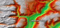
Hiking Trail Planning – The “cost” would be very different for planning a family-friendly hiking trail. In this case, you would want to build it on the least amount of slope so it’s safe to climb. As you go from the start point to its destination, you want to “buy” the lowest “cost”, which would be the least amount of slope. Any route to the top equals the same net change in elevation. But the least cost path accumulates the least amount of slope from start to finish.
How To Use the Least Cost Path
There are three main steps when you run this analysis:
- Cost distance – First, you have to calculate the cost in relation to your start point. For routing a hiking trail, your cost matrix would be the slope. The higher the slope, the more costly it would be.
- Cost backlink – Second, you need to calculate the raster backlink. In this case, it would be the direction in which the path will go with all 8 possible cardinal directions from one cell to the next.
- Cost path – Finally, you can calculate it using the cost distance, cost backlink, and destination source. No matter which route, any path to the destination equals the same net change in elevation. But it accumulates the least amount of slope.
The result is the most cost-effective route from the starting point to the final destination. Here’s a video that describes LCP in ArcGIS Pro using weight, barriers, and a bit of ModelBuilder.
Summary: Least Cost Path
The least cost path may be one of the best tools in the GIS arsenal for any linear infrastructure and routing application.
But the key is that your input data are all logical, accurate, and complete.
Only then can it determine the most cost-effective path by accumulating the least amount of “cost”.
Do you want to try out more raster analysis tools? Then, here are some more that can help you become a raster master:


Hello, please I would like to know an example of local geographic phenomena in Ghana and its explanation in terms of source raster, cost raster, and cost distance measure, thank you.
Hi
In the Least Cost Path method, is it possible to select a maximum slope of 10% for route design?
Also, the path that he suggests should be close to the criteria of Road or Highway (for example, longitudinal slope, geometric and Curve design, etc. are suitable), not walking!